Replies

Hi Zeddy et al

This is my attempt to address the shortcoming that Zeddy identified whereby replacements were not context sensitive. This meant that the colour red would update in both the colour and status contexts. The latter being inappropriate.

The following line checks the validation formula for the appropriate table name in the validation source.

Code:

                [COLOR=#b22222]If InStr(ActiveCell.Validation.Formula1, sTblSrcName) Then[/COLOR]

The variable sTblSrcName is populated by the routine named getSrcTableName.

I am still having trouble implementing Cells.SpecialCells(xlCellTypeSameValidation). It does not seem to like the event trigger location.

Code:

Public sTblSrcName As String

Sub upDateValidation(sOldValue As String, sNewValue As String)
    Dim rng As Range
    Dim oCell As Range
    On Error GoTo ErrorTrap
    Application.ScreenUpdating = False
    getSrcTableName
    For i = 2 To Worksheets.Count
        Sheets(i).Activate
         '**Get all cells with validation set
        Set rng = Cells.SpecialCells(xlCellTypeAllValidation)
'        Set rng = Cells.SpecialCells(xlCellTypeFormulas)
'        Set rng = Cells.SpecialCells(xlCellTypeSameValidation)

      On Error GoTo 0
            For Each oCell In rng
            oCell.Select
                oCell.Validation.IgnoreBlank = False
                'test tableName in validation formula
                [COLOR=#b22222]If InStr(ActiveCell.Validation.Formula1, sTblSrcName) Then[/COLOR]
                    If oCell.Value = sOldValue Then oCell.Value = sNewValue
                End If
            Next
    Next
    Set rng = Nothing
    MsgBox ("All Done")
    Exit Sub
ErrorTrap:
     MsgBox "There is an error " & Err.Description
     
End Sub

[COLOR=#b22222]Sub getSrcTableName()[/COLOR]
For i = 1 To ActiveSheet.ListObjects.Count
    If Not Intersect(ActiveCell, Range(ActiveSheet.ListObjects(i))) Is Nothing Then
        sTblSrcName = CStr(ActiveSheet.ListObjects(i).Name)
'        Debug.Print sTblSrcName
        'sTblSrcName = getSrcTableName
        Exit Sub
    End If
Next

End Sub

Thanks to Zeddy and Fred for their comments and assistance to date.

Geof

Hi Fishunt

Welcome to the world of the balding.

A bit of background on Vlookup()
By design only 3 of the 4 arguments :- target, Lookup table, and column position of desired data are required.

By design and default Vlookup() will return a match based on the value that is either equal to target OR nearest to and smaller than target.

When you append the fourth argument and specify “False” you are instructing the function to force an exact match for the target data. .. instead of nearest to or smaller than target.

By default and design the function expects that column 1 of the lookup table to be sorted in ascending order.
This is easy to spot with numeric data but a tad more tricky with alphanumerics. ( “a1” is not the same as “a 1”)

Use of alphanumeric data in column 1 of the lookup table is an additional reason to specify the “false” in the 4th argument.

The inclusion of “False” as argument 4 solved your problem as it negated the default behaviour of the vlookup().

On a copy I would suggest observing the effects of sorting your lookup table by col 1 just for your education.

Zeddy makes a good point by naming the block. It makes the formula far easier to read.

Have a look at the MS support site for more information.
Hope this helps in the future.

G

Hi
I sometimes find it easier to get things working chunk by chunk.
Try this after changing tweetyBird’s email address.

Code:

Sub sendEmail()
'skeleton test script from Excel vba
Dim oApp As Object
Dim oMail As Object

Set oApp = CreateObject("Outlook.Application")
Set oMail = oApp.CreateItem(olMailItem)
'Set oMail = oApp.CreateItem(0)
    With oMail
        .to = "tweetyBird@gmail.com"
        .CC = ""
        .BCC = ""
        .Subject = "This is the Subject line"
        .Body = "Hi there from Daffy Duck"
        .Send   'or use .Display
        '.display
    End With
End Sub

Hope it helps
Geof

Hi
Changes made include

[*]Cycling through the Validated Cells collection. No longer using .UsedRange.
[*]Using 2 validation sources in the Lists sheet.

It should operate more quickly now.
Cheers
Geof

Hi Fred
The empty sheet was only there to check for bugs if sheet was empty. It is not required at all. I forgot to delete it.

I cant get it to reliably mark invalid data with circles if I play around deleting items from the data table.

A blank cell updates in the validation list, and updates the validated cells to blank… most of the time.

Deleting a row from the table leaves the validated cells alone, the validation list updates for you to access with the drop list. But I cant mark the validated cell as invalid with .circleInvalid.
Which is why I haven’t used it.

As I said .. problem between the keyboard and back of my chair.
G

Cheers
Geof

Hi folks
The attached workbook is my attempt to automate the updating of validated cell contents in the event that you edit the validation source list.
I have used an Indirect() function against a list range converted to a table to maintain a dynamic range. I am trying this as an alternate method to using the Offset() function. The Indirect() formula in the validation is easier to read.
The scripts require that the worksheet named “Lists” remains at the first worksheet in the workbook.
There are two routines behind the worksheet named “Lists”.

[*]Worksheet_Change and
[*]Worksheet_selectionchange.

These routines capture the events and use the Intersect method to monitor changes. They capture values necessary as inputs to the upDateValidation routine in Module1.
These routines came from the microsoft support site.

Module1 contains two scripts

[*]upDateValidation() and
[*]isValidated()

IsValidated() tests whether cells are subject to data validation.

I have no idea if this is at all useful. It seems to work with a very small sample workbook. It has proved to be an interesting problem. On the face of it capturing selection changes and workbook changes could be annoying !!

Zeddy
I could not get the activesheet.circleInvalid to work for me !? Problem must be between the keyboard and the back of the chair.

Known Issues

[*]Deleting a row from the table data source.
[*]Deleting cell contents from table data source

Cheers
Geof

Hi again

Dynamic Range Names & use of Offset()

Are there advantages to this function over the use of a range converted to a table?

A Data Validation rule could reference a table name instead

Something like this :- =INDIRECT(“Table2[Town]”)

To my aging eyes this is a lot easier to read.

Just wondering. Legacy issues?
Geof

Hi folks
Thank you .. every day is a school day.

activesheet.circleInvalid is indeed new to me.

Geof

Hi Wayne
In a spreadsheet it is possible to suppress the view of rows or columns. In doing so the data and relationships are preserved.
Hide a column
Easiest way to hide a column is to right-click on the column header and select HIDE from the context popup menu.
Unhide
Select a columns each side of the where the hidden col would be, right click and select UNHIDE.

Of course you could store the initial data in my example B1 somewhere entirely different/off-screen and make a formula in B1 reference the new off-screen location. The formula in B1 would thus be =If(a1=””,?,?+1), where ? stands for the off- screen cell location.

The same concerns about behaviour after editing A1 still apply.
Cheers
G

Hi Wayne
Are you able to introduce an extra column into the model as in attached screenshot? In this scenario the formula is in C1 and I would hide the intermediate column B.

But what happens if you subsequently change the value in example A1?

42157-wayne1

Hi folks
I started playing as a learning exercise.
Is there any merit in the following approach?
This is not offered as a solution but more for comment as part of my learning. There will be bugs.

The intent is to loop through cells in the usedRange. (problem #1 I guess)
On each pass check for validation and if conditions are met substitute old value for new value.

As it stands the new value could fail the validation.

42153-validations

Code:

Sub Test()
CheckValidation "red", "green"
End Sub

Sub CheckValidation(sOldValue As String, sNewValue As String)
Dim oCell
For Each oCell In ActiveSheet.UsedRange
    oCell.Select
    With ActiveCell
        If isValidated And .Value = sOldValue Then .Value = sNewValue
    End With
Next
End Sub

Function isValidated()
Dim X As Variant
On Error Resume Next
isValidated = True
X = ActiveCell.Validation.Type ' eight types values 0 to 7
On Error GoTo 0
If IsEmpty(X) Then
    isValidated = False
End If
End Function

Comments are most welcome.
Regards
Geof

Hi

the VBA equivalent of CurrentRegion

If for some reason you did not want to use an explicit cell reference you could try something like this

ActiveCell.CurrentRegion.AutoFilter field:=1, Criteria1:=”yourCriteria”

I am not sure of advantages / disadvantages of either method for you.

Cheers
G

Hi
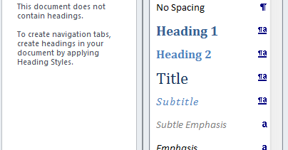
Are you describing a version of Word with the ribbon interface? If this is the case does this

not being the quick style toolbar

refer to the Quickstyle Gallery ?

42130-TaskPanes
The image above shows the navigation and the Styles Pane in my Word 2010.

You are able to customise the Styles pane to your heart’s content.

For information about this check out this site.

I hope this helps.
Geof

Hi

I am guessing that someone has missed an apostrophe to comment out the “0” Or “123”.
Hence coding error.

I wonder if the code runs because the value component of the variables.add method is optional.

I tried this quickly

Code:

Sub test()
ActiveDocument.Variables.Add "Office", "0" Or "123"
End Sub

Sub test2()
For Each oVar In ActiveDocument.Variables
    Debug.Print oVar.Name & vbTab & oVar.Value
Next
End Sub

The printed result read Office 123

Cheers
G

Hi again
Yet another approach

Text To Columns
You will find this on the data tab in Excel.

This tip assumes that you can edit the Excel data source.

Text To Columns enables you to split the contents of a single cell across multiple cells within the same row. The split is based on a specified delimiter. In your example the delimiter is the period.

You nominate the cell address that marks the beginning of the output target range. Take care to avoid overwriting existing data.

G