Trying to calculate income spread across months

Topic

New Reply

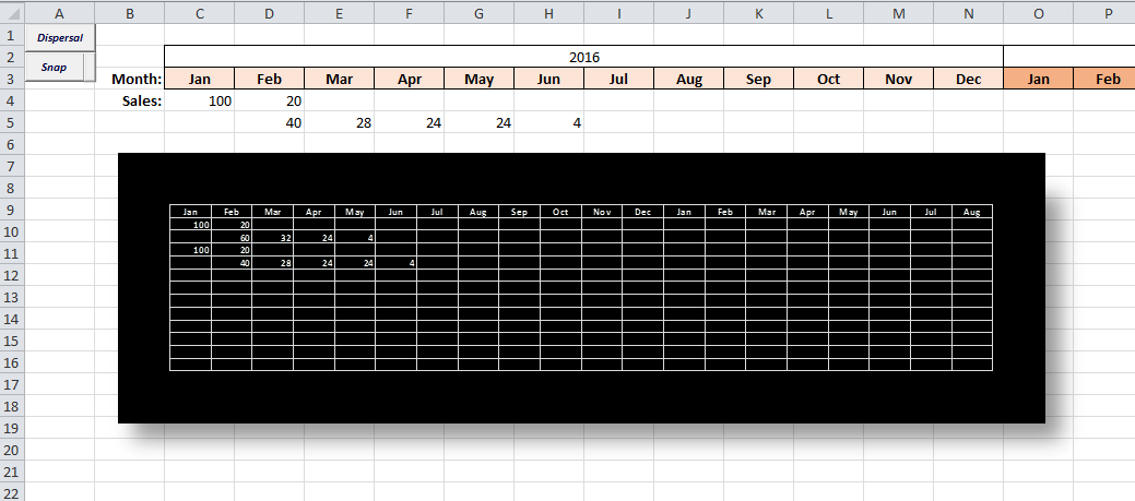
I have a sheet that looks like the below. We close a sale and 30 days later we start work. I want to spread the sale amount over four months (average time across varying size projects) for cash flow analysis. And show the total expected to invoice for each month based on that. I show in the example only a few months. Hope you get the picture. I’m looking for a formula for the second row to do the calculation. I’m getting nowhere with this!
I see the table isn’t showing so adding an attachment.

[TABLE=”class: grid, width: 500″]
[TR]
[TD][/TD]
[TD]Jan[/TD]
[TD]Feb[/TD]
[TD]Mar[/TD]
[TD]Apr[/TD]
[TD]May[/TD]
[TD]June[/TD]
[TD]July[/TD]
[/TR]
[TR]
[TD]Projected Sales[/TD]
[TD]45000[/TD]
[TD]90000[/TD]
[TD]135000[/TD]
[TD][/TD]
[TD][/TD]
[TD][/TD]
[TD][/TD]
[/TR]
[TR]
[TD]Projected Invoice Amt[/TD]
[TD][/TD]
[TD]45000/4[/TD]
[TD](45000/4)+(90000/4)[/TD]
[TD](45000/4)+(90000/4) + (135000/4)[/TD]
[TD](45000/4)+(90000/4)+ (135000/4)[/TD]
[TD](90000/4)+ (135000/4)[/TD]
[TD](135000/4)[/TD]
[/TR]
[/TABLE]

Reply | Quote

Replies

Not sure I fully understand.

Do you want the first calc in column D row 2 to be: =0.25*SUM($C$4:C4) ? Then, fill that across 3 columns.
Then, in G: =0.25*SUM(C4:$E$4) and fill that across three?

Reply | Quote

Was hoping to figure out how to do it all in one formula, one row, handling how many ever months there are. Something that could count the number of times the sales amt had been used then drop it.

Reply | Quote

OK, it’s 5 minutes later and the brain is starting to function.

To adjust for the -4, try:

=SUM(INDIRECT(“R4C” & COLUMN()-IF(COLUMN()<5,COLUMN()-1,4),FALSE):INDIRECT("R4C" & COLUMN()-1,FALSE)) / 4

Personally, I think this is messy just to account for the fact of where you started your data. I'd move the column of labels to col D so that your first month's data is in col E. But that's me.

Also, if for whatever reason you decide to do away with the column of labels and start your data in col A, then the "-1" part towards the end would also become a problem. Sounds like that won't happen but I think you can see how to adjust the formula if you decide to do that.

Fred

Reply | Quote

how about a formula like:

=SUM(INDIRECT(“R4C” & COLUMN()-4,FALSE):INDIRECT(“R4C” & COLUMN()-1,FALSE)) / 4

Put this in row 5 (or some other row) and fill across.

The only (?) problem with the formula is that you can’t start it before column E (ie, it won’t work in columns A-D) because the “COLUMN()-4” part looks 4 columns to the left of the present column. There is no column 4 columns to the left of D.

An easy solution would just be to start your data so that Jan is in column E.

I think with a little more work, I could avoid that restriction also. Just need to work on the “-4” part a little. But it’s early here and my brain still isn’t fully awake.

Fred

Reply | Quote

ok. very cool. thanks. now I get to try and figure out how this works!
it’s a bit hard to move the data as it gets swept into our forecast tool, but I’ll try moving everything to E and see if I can remap the import

Reply | Quote

I don’t know if you saw my second post.

There is no need to move the data to start in col E if you use the revised formula of my second post.

You mentioned in post #3 that you wanted a single formula, so this will do it.

But with your data beginning in col C but you wanting the previous FOUR months, that creates a problem (referring back 4 cols) until you get to col E.

For example, if your data began in col C but you only wanted to go back 2 cols (sum up cols A and B), there would be no problem. If your data began in col E but you wanted to sum up 5 months, there would be a problem.

The problem, generally, is that you can NOT go back past (to the left of) col A.

From a purist point of view, the formula of post #5 is a bit messy. Compare the formula in post #4 vs #5 (when I was awake). The only difference is that -4 in the first one is replaced by that
-IF(COLUMN()<5,COLUMN()-1,4)

Note what the -IF does: if the column where you want to start the sum is less than 5 (columns, although usually identified by a letter, can also be referenced by the corresponding number – col A is 1, col B is 2, etc) meaning to the left of E, then we do NOT subtract 4 since that would take us back beyond the left of col A (which is NOT allowed, equivalently a col with a number of 0 or less). Instead we start the sum from col A (or the first col).

If the column where you want to start the sum is 5 or more (col E and beyond to the right), then the test
COLUMN()<5
is false, and the result of -IF will always give 4.

So if you look at the 100th or 952nd or 2500th col, the -IF is always FALSE and you're always starting the summing 4 cols to the left of the present column. At this point, you might wonder why the -IF is there, rather than just a 4.

The present column where you're putting the formula has a col given by COLUMN(). We don't have to actually know which column we're in to reference the current column.

So, I think your options are
1) move the labels to col D and start the data in col E; then you can use the formula in post #4 EVERYWHERE.
At this point, it could also be simplified to something like

SUM(A4: D4)/4 for col E.

As you fill to the right, Excel will adjust the formula to SUM(B4:E4)/4 for col F, then SUM(C4:F4)/4 for col G, etc.

2) if you want to keep the labels in col B, then
2A) use the formula in post #5 everywhere or
2B) use the formula in post #5 for just col D (and col C if you want) but then use the formula in post #4 from col E forever to the right.

As to the rest of the formula, the 2 INDIRECTs are putting together a starting point and an ending point for summing. Since these change with every column, you can't have a fixed column reference. That's what the COLUMN()-4 and COLUMN()-1 do. When added to the end of (concatenated with) the fixed string "R4C", you get something like R4C2 for a start and R4C5 for an end. (This is an alternative form of referencing cells called "RC" referencing, where you give the Row # after the "R" and the Col # after the "C" all as one string.)

Note that the 4 is because your sums are in Row 4. If you change your mind for this, you'd have to change the 4 to the proper row # (there are other alternatives than using a constant row # but those really don't seem to be needed here based on what you originally posted).

Hope this helps.

Fred

Reply | Quote

Hi Fred or anyone!
So this solution has worked very well and now it’s time to improve. I need a kick start! The current formula looks at the past 4 months and uses 25% from each month to create the total. Perfect. But what if I want to have this more dynamic. Say spread the income 30%/30%/20%/20% instead. Or spread it out across five months instead of four. Can the formula be modified to do a lookup for number of months to use and % for each month?

I don’t know if you saw my second post.

There is no need to move the data to start in col E if you use the revised formula of my second post.

You mentioned in post #3 that you wanted a single formula, so this will do it.

But with your data beginning in col C but you wanting the previous FOUR months, that creates a problem (referring back 4 cols) until you get to col E.

For example, if your data began in col C but you only wanted to go back 2 cols (sum up cols A and B), there would be no problem. If your data began in col E but you wanted to sum up 5 months, there would be a problem.

The problem, generally, is that you can NOT go back past (to the left of) col A.

From a purist point of view, the formula of post #5 is a bit messy. Compare the formula in post #4 vs #5 (when I was awake). The only difference is that -4 in the first one is replaced by that
-IF(COLUMN()<5,COLUMN()-1,4)

Note what the -IF does: if the column where you want to start the sum is less than 5 (columns, although usually identified by a letter, can also be referenced by the corresponding number – col A is 1, col B is 2, etc) meaning to the left of E, then we do NOT subtract 4 since that would take us back beyond the left of col A (which is NOT allowed, equivalently a col with a number of 0 or less). Instead we start the sum from col A (or the first col).

If the column where you want to start the sum is 5 or more (col E and beyond to the right), then the test
COLUMN()<5
is false, and the result of -IF will always give 4.

So if you look at the 100th or 952nd or 2500th col, the -IF is always FALSE and you're always starting the summing 4 cols to the left of the present column. At this point, you might wonder why the -IF is there, rather than just a 4.

The present column where you're putting the formula has a col given by COLUMN(). We don't have to actually know which column we're in to reference the current column.

So, I think your options are
1) move the labels to col D and start the data in col E; then you can use the formula in post #4 EVERYWHERE.
At this point, it could also be simplified to something like

As you fill to the right, Excel will adjust the formula to SUM(B4:E4)/4 for col F, then SUM(C4:F4)/4 for col G, etc.

2) if you want to keep the labels in col B, then
2A) use the formula in post #5 everywhere or
2B) use the formula in post #5 for just col D (and col C if you want) but then use the formula in post #4 from col E forever to the right.

As to the rest of the formula, the 2 INDIRECTs are putting together a starting point and an ending point for summing. Since these change with every column, you can't have a fixed column reference. That's what the COLUMN()-4 and COLUMN()-1 do. When added to the end of (concatenated with) the fixed string "R4C", you get something like R4C2 for a start and R4C5 for an end. (This is an alternative form of referencing cells called "RC" referencing, where you give the Row # after the "R" and the Col # after the "C" all as one string.)

Note that the 4 is because your sums are in Row 4. If you change your mind for this, you'd have to change the 4 to the proper row # (there are other alternatives than using a constant row # but those really don't seem to be needed here based on what you originally posted).

Hope this helps.

Fred

Reply | Quote

I’m looking for the post I just made in response so I could edit it but can’t find it. So I’ll try again.

NOTE: I just found my previous post and deleted it. This new post is more direct.

In your original spreadsheet, you had sales for each month. One might assume that the total sales figures are the result of several sales.

So when you ask about changing the rule of “spread each month’s sales over 4 months evenly”, would it be safe to assume that you want to change the rule to the total sales? Doing otherwise (changing the rule on a per-sale basis) doesn’t seem feasible since your original spreadsheet did not go to that level of detail.

Also, when you ask about changing the rule, I’d assume that the change would apply to all months. Is that true? Or would you want the sales of some months to be treated differently than for other months. In other words, could you have the sales in Jan spread over 4 months but the sales of Feb spread over 5 months? Same question applies to the percentages (sales for Jan treated evenly but for Feb treated as 30-30-20-20).

Lastly, do you want to be able to compare, in one spreadsheet, the cash flow for different rules? Or just apply a rule, look at the result, maybe print it out, and then just do another rule? It would seem that some place is needed to store the different rules regardless of your answer. It would also seem that a VBA solution might be needed.

Depending on your answers, I’m thinking this is getting beyond my skills (and it’s still early here so my brain is not awake). But I’ll bet that Maud, RG, Zeddy and others would be able to help.

Fred

Reply | Quote

Right. I’m not trying to make a big leap. So not project by project and same rules for entire forecast. Just total sales for the month like last time. In line answers below in CAPS

I’m looking for the post I just made in response so I could edit it but can’t find it. So I’ll try again.

NOTE: I just found my previous post and deleted it. This new post is more direct.

In your original spreadsheet, you had sales for each month. One might assume that the total sales figures are the result of several sales. TRUE

So when you ask about changing the rule of “spread each month’s sales over 4 months evenly”, would it be safe to assume that you want to change the rule to the total sales? Doing otherwise (changing the rule on a per-sale basis) doesn’t seem feasible since your original spreadsheet did not go to that level of detail. CORRECT. MAYBE BY TYPE OF PROJECT NEXT YEAR

Also, when you ask about changing the rule, I’d assume that the change would apply to all months. Is that true? Or would you want the sales of some months to be treated differently than for other months. In other words, could you have the sales in Jan spread over 4 months but the sales of Feb spread over 5 months? Same question applies to the percentages (sales for Jan treated evenly but for Feb treated as 30-30-20-20). SAME NUMBER MONTHS FOR ENTIRE FORECAST

Lastly, do you want to be able to compare, in one spreadsheet, the cash flow for different rules? Or just apply a rule, look at the result, maybe print it out, and then just do another rule? It would seem that some place is needed to store the different rules regardless of your answer. It would also seem that a VBA solution might be needed. I’M GOOD WITH ONE SHEET, ONE RULE, ONE FORECAST.

Depending on your answers, I’m thinking this is getting beyond my skills (and it’s still early here so my brain is not awake). But I’ll bet that Maud, RG, Zeddy and others would be able to help.

Fred

Reply | Quote

bdesilva

A VBA approach. Here is some code that will update the invoice values with no formulas when a new sales value is entered. The values will also be updated if you remove the values. Place the code in a worksheet module.

HTH,
Maud

Code:

Private Sub Worksheet_Change(ByVal Target As Range)
[COLOR=”#008000″]’—————————————-
‘SETUP ERROR TRAPPING[/COLOR]
On Error GoTo Enable
Application.EnableEvents = False
[COLOR=”#008000″]’—————————————-
‘DECLARE AND SET VARIABLES[/COLOR]
Dim LastCol As Integer, I As Integer, J As Integer
Dim SalesRow As Integer, StartSalesCol As Integer, rng As Range
SalesRow = 4
StartSalesCol = 3
LastCol = ActiveSheet.Cells(SalesRow, Application.Columns.Count).End(xlToLeft).Column
[COLOR=”#008000″]’—————————————-
‘CLEAR INVOICE VALUES PRIOR TO CALCULATIONS[/COLOR]
ActiveSheet.Range(Cells(SalesRow + 1, 3), Cells(SalesRow + 1, ActiveSheet.Cells(SalesRow + 1, _
    Application.Columns.Count).End(xlToLeft).Column)).ClearContents
[COLOR=”#008000″]’—————————————-
‘LOOP THROUGH SALES AND UPDATE PAYMENTS OVER NEXT 4 MONTHS[/COLOR]
For I = StartSalesCol To LastCol
    If Cells(SalesRow, I)  “” Then
        For J = 1 To 4
            Cells(SalesRow + 1, I + J) = Cells(SalesRow + 1, I + J) + (Cells(SalesRow, I) / 4)
        Next
    End If
Next I
[COLOR=”#008000″][/COLOR][COLOR=”#008000″]’—————————————-[/COLOR]
Enable:
Application.EnableEvents = True
End Sub

Reply | Quote

Thanks Maudibe. That’s a cool approach I’ll review tonight.
Thanks Fred so much for all that detail. I’ve learned a lot today!

Reply | Quote

Still early in the morning – for me. So remember that the brain may not be fully awake yet.

Before trying a solution, I’d have to ask some questions.

Are you changing the rule of “spread cash flow EVENLY over 4 MONTHS” for every job or on a job-by-job basis? It sounds like the former but I’d want to ask.

In other words, could some jobs be over 3 months while others are over 5? Could some jobs for 4 months have cash flows evenly while others over 4 months be 30-30-20-20?

Or are you trying to see, if for ALL jobs, you change the current rule to compare how that affects cash flow?

If each job can have a different rule, where will that information come from? Would you create a sheet of “rules” where each rule has a #months and % of price due each month? Then for each job, you’d just need to refer to the proper rule.

If you change the rule for all jobs, would you want to have in your one spreadsheet a comparison of the cash flow for all rules?

I’m not sure I’d be able to help depending on the answer (and almost definitely not today as I have a full plate of things to do). But I’d bet on Maud, RG, Zeddy, or others being able to move this along depending on the answers.

Also note that my questions above are just what I think needs answering before beginning a solution. Others might need clarification along related lines.

Fred

Reply | Quote

Maud, RG, Zeddy, fburg?? Any ideas appreciated. I’m just not getting anywhere on my own.

Reply | Quote

Attached is a spreadsheet that only takes into account a change to the # of months over which the sales are counted. This looks like it should work but I only did limited testing. You should definitely do a bit more testing with your data.

Note I put in the # months in B1 (and put a label in A1). This is used in the calculations.

Also note that I did not account for any potential rounding effects. For example, if Jan sales = 100 and that is to be spread over 3 months, then Jan will be counted as 33.3333 for the next 3 months. This could be rounded but then each of the 3 months would be 33.33 or 33.34. Rounding so that the first 2 months are 33.33 and the last month is 33.34 would be harder.

I left the rows for your original explanation but moved these rows down just to be out of the way. However, they are no longer correct (or needed?) if the # months is not 4.

Being able to change the % allocation per month to NOT be the same each month (as opposed to keeping it equal based on the # months, which is what I did) would be harder – perhaps not even doable without VBA. Perhaps a modification to the code that Maud posted? I looked at his code and it doesn’t look too difficult to modify for both features (# months, unequal %). However, I won’t be able to get to either approach (unequal % with or without VBA) today.

Is there some # of MAXIMUM months over which the sales would be spread? I’m thinking of a non-VBA solution where I’d have “helper” rows (rows where intermediate calculations are done rather than trying to capture everything in 1 formulas) for each of those months. If the maximum number of months is NOT used, then those rows would be 0. Then there’s be 1 more row to sum all the helper rows, which is what you want. If necessary, the helper rows can be hidden.

Fred

Reply | Quote

Arrg. Swear I answered this ten minutes ago but cannot find it!
Thanks again Fred. I’ve added the change to my model and it works. I’ll take a lot at the VBA tonight and see what I can make of it. Haven’t done programming stuff for over a decade though!
For the short term I’d say the maximum spread will be 9 months. Ultimately I’d like to change it based on what accounting shows really happens post forecast but I haven’t done enough research to know what that is! So if I could spread 4-9 months that’d be enough for 2016!

Reply | Quote

Brian,

I amended the code to accommodate the payments spread out up to nine months and nine different available percentages in 5% increments. Click on the dispersal button to open the Invoice form. Select the number of months. The number of enabled percentages adjusts to how ever many months to spread the payments. Select the percentage for each available month. The Remaining % textbox tracks the total percentage and remains red until the total remaining percent equals zero. When you have the spread set the way you desire, click save. The form will close and you can make your entries. The form will also remember your settings.

HTH,
Maud

44647-Dispersal2

Reply | Quote

I knew Maud could do it!

A few comments:
– I changed the # months to 6, decreased one of the month’s allocation, and put the remaining % in month 6. I observed that the current allocations did not change. I would think that given a set of sales, one might want to play around with the monthly allocations to see how the cash flow is affected. That is, once the dispersal form is saved, the cash flows in row 5 should be updated. But that is for the O.P. (original poster) to comment on.

– I also observed, while changing the # dispersal months to 6, that I could put in a % into month 6 that created a sum > 100% (even with the remaining % to be allocated now shown in red). Again, it should be clear to a user that this should not be. But it would seem a warning about allocating >100% should be issued and, perhaps, you NOT be allowed to save the form – especially if the %s are used to update the cash flows per above.

– Lastly, with the current allocations as created in Maud’s file, I’m not sure if the cash flows are adding up correctly.
— For Jan, sales = 100. So for Feb, cash flow is 15%*100=15. No problem.
— For Feb, new sales=20. So for March, cash flow should be (Jan’s sales with Month 2’s allocation) + (Feb’s sales with Month 1’s allocation). Assuming this is correct, that gives 30%*100 + 15%*20=30+3=33. No problem.
— For March, no new sales. So for April, cash flow should be (Jan’s sales with Month 3’s allocation) + (Feb’s sales with Month 2’s allocation). This should give 35%*100 + 30%*20 = 35+6 = 41. Results are showing 46 ????

I could also see, perhaps as part of my first dash, that once a set of dispersals is saved, that the %s should be put into some (protected?) set of cells so one can see how the cash flows change as the % allocation changes WITHOUT having to call up the form. Not that calling up the form is hard, but it could be desirable to copy/paste the info to another sheet showing dispersal %’s, sales, and cash flows for some subset of months. Again, something for the OP to comment on.

I may have some time over the next few days to create a non-VBA solution along the lines that Maud did. There would be a set of cells to enter %s into, like Maud’s form, and a check to see if they add up to 100%. The cash flows could then be calculated, perhaps using helper (hidden) rows, as suggested in my previous post. Whether this is still needed, in light of Maud’s excellent solution, is something that I’d wait on guidance from the O.P.

Fred

Reply | Quote

oh my how beautiful this is! So I need just a little help getting it in my spreadsheet. How do I move what I need into my workbook, and how do I make it use the rows/columns of my model?

Reply | Quote

– I changed the # months to 6, decreased one of the month’s allocation, and put the remaining % in month 6. I observed that the current allocations did not change. I would think that given a set of sales, one might want to play around with the monthly allocations to see how the cash flow is affected. That is, once the dispersal form is saved, the cash flows in row 5 should be updated.

Making any change to the Invoice form will update the dispersal when the next sales entry is placed. Fred makes a good suggestion to update with any form change. I will make the simple tweak.

– I also observed, while changing the # dispersal months to 6, that I could put in a % into month 6 that created a sum > 100% (even with the remaining % to be allocated now shown in red). Again, it should be clear to a user that this should not be. But it would seem a warning about allocating >100% should be issued and, perhaps, you NOT be allowed to save the form – especially if the %s are used to update the cash flows per above.

Fred, Maybe you didn’t try to save when the percentages didn’t add up to 100%. Not only will the total percentage stay red but you will not be able to save and you will be presented with a message stating such. This will occur if the total percentage is less than as well as greater than 100%. Note: saving the Invoice form saves only the form settings, not the workbook.

44655-Dispersal4

– Lastly, with the current allocations as created in Maud’s file, I’m not sure if the cash flows are adding up correctly.

Fred, I played with this extensively and I believe my code calculates spot on. Using a dispersal over 5 months with a spread of 15%, 30%, 35%, 15%, and 5% the image below shows the breakdown verifying that the code calculated correctly> Perhaps we have a different interpretation on how the calculations should be performed

44654-Dispersal3

oh my how beautiful this is! So I need just a little help getting it in my spreadsheet. How do I move what I need into my workbook, and how do I make it use the rows/columns of my model?

Brian, the simplest way is to post or email me your finished blank file and I will insert all the code for you. Otherwise, I will need to provide explicit instructions on how to import the code. I will also need to create a “setup form” so that you can configure the code for your sheet. Either way, I will need a finished but blank file.

I will post a new file coded with Fred’s suggestion to update the totals when the Invoice form is updated.

Hope this all helps,
Maud

Reply | Quote

Brian,

Fred had some great ideas. This revision employed two of them
1. The Sales and Payments will update on the Analysis sheet if changes on the Invoice Form are saved.
2. You can “snap” the Sales and Payments to a holding grid for comparison while running a new set of numbers. Next to the “Snap” button is a narrow button to clear the grid.

Let me know if you need help if you choose to use this code in your project

Maud

44657-Dispersal5

Note: This was created in Excel 2010

Reply | Quote

I surely need help 😉
I have a mock up file I’m using already that I can email if you tell me where, although I’d love to see what you have to do so I understand it. But you’ve already done so much just whatever is easiest.

Reply | Quote

Hi Maud,

Fred, Maybe you didn’t try to save when the percentages didn’t add up to 100%.

You’re right. I had thought the error msg would come up as soon as the totals showed other than 100%. I didn’t include “less than” 100% because that’s certainly possible while you’re first filling the percentages. Of course, no single month could be negative or greater than 100 since those are not choices in the drop-down box. So I can see the error msg being useful only when you go to Save the form. But certainly it’s possible to catch the error as soon as it occurs, rather than waiting for one to save the form, if a % selection sends the total over 100. But I don’t think it’s a big deal.

Fred, I played with this extensively and I believe my code calculates spot on.

I looked at your very cool “arrow” diagram showing the calculations.
– First, if there’s some tool you use for this, please advise where to find since I could use that for lots of things. If not, you sure spent a lot of time making that diagram – very nice!
– Second, my calculations in my previous post did agree with your arrow diagram. And my method did agree with it too. BUT I downloaded a fresh copy of your previous version (the one I had commented on) just to be sure my copy was not messed up. See attached screen shot on what I got for April (the 46 for April, rather than the 41 which I calculated and your new version is getting).

Reply | Quote

Maud,

I just tried your new version. Very cool.

I almost didn’t see the narrow button next to the Snap button. Could be worsening eye sight with advancing age.

Very cool that the grid allows comparison of different dispersal strategies. I assume it also allows different sales to be saved too but I didn’t trying changing the original sales. I guess when you “snap”, the grid stores the current sales values in row 4 and the current cash flows from row 5.

Fred

Reply | Quote

Brian,

Click on your “Settings” at the top of this page > General Settings > Tick “Private Messaging On” and “From all Members. Also check “Receive email from other members”. I will PM you my email address or you can email me by left clicking on my name above my avatar from within a tread. I’ll be happy to introduce the code into your workbook and heavily comment the lines so you can follow what it is doing.

Maud

Reply | Quote

Bryan,

Thanks for the file you sent. I have integrated the code, forms, and grid into your spreadsheet. Because many of your sales values are calculated from another sheet. I had to use the Workbook_SheetChange event to capture a change from any sheet

Code:

Private Sub Workbook_SheetChange(ByVal Sh As Object, ByVal Target As Range)
[COLOR=”#008000″]’ANY CHANGE ON ANY SHEET UPDATES INVOICES[/COLOR]
Application.EnableEvents = False
    UpdateInvoice
Application.EnableEvents = True
End Sub

Because there was a need to toggle the Application.EnableEvents off/on, I placed a reset button on the sheet to turn it back on if something goes awry.

44685-bdesilva1

Some other new additions are the Settings Form which will allow you to customize your sheet if you move rows and columns. Selecting a setting will open a description of what the setting does in the adjacent text box

44686-bdesilva2

You will also notice that I added additional columns for the successive year. They will be needed if the invoice spreads beyond Dec 31 (see row 13). Additionally, the grid extends a successive year as well while both retain the year end total column. To assist you, I have commented nearly every line

I have emailed the file to the address you provided. Let me know if you need additional assistance.

Maud

Reply | Quote

Thanks! I’ll review this afternoon. As I said before, you are awesome!

Reply | Quote