Excel 2013/2016: How to Save Picture In Cell To Disk

Topic

New Reply

Hi,

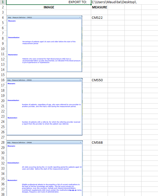
I searched the forums, but came up empty. In Excel, I have a worksheet with images appearing in one column and a numerical identifier in another column. I want to create a macro that will export the images to disk using the associated identifiers as the file name. Sounded simple, until I discovered that images are not part of the cell, but of the worksheet and are basically anchored to a cell, so querying each cell to get the picture does not work.

I can successfully loop through the worksheet shapes, get each image, and copy it to the clipboard (using Cells(range).CopyPicture), but cannot see how to save it to disk. I would also have to use something like “Shape.TopLeftCell.Address” to determine which row it is anchored to in order to get the associated identifier.

I tried using VB6 to do the same thing and got just as far — can copy to the clipboard — but when I try to use SavePicture I get an error about Invalid Property Value.

Before I bang my head any further, is there some way that I have been overlooking to accomplish this seemingly simple task?

Thanks!

Reply | Quote

Replies

Hi generic,

This can be done by adding a pic to a chart (background) then saving the chart as a .gif.

The following code cycles through the images in col A, grabs the file name in adjacent column B, and then copies the image. The code then creates a chart sheet and pastes the image into the chart and finally saves it as a .gif using the path in cell B2 and the captured file name.

Note: Change the name of the path in cell B2. If you use my method to capture the pic names and to copy the pics to the clipboard, make sure that the top of each image is within the row that the image name is located. The code assumes that the row height is consistently 15 and the only shapes on the sheet are the images. If you want to add buttons then while looping through the shapes on the sheet you will need to add code to test for the type of shape

HTH,
Maud

Code:

Public Sub SavePic()
    Application.ScreenUpdating = False
    Application.DisplayAlerts = False
[COLOR=”#008000″]’———————————————‘
‘DECLARE AND SET VARIABLES[/COLOR]
    Dim Pic As Shape, PicTop As Double, Row As Long, Path As String, fname As String
[COLOR=”#008000″]’———————————————‘
‘LOOP THRU IMAGES ON WORKSHEET AND GET FILE NAME[/COLOR]
    For Each Pic In ActiveSheet.Shapes
        PicTop = Pic.Top
        Row = WorksheetFunction.RoundUp(PicTop / 15, 0)
        Path = Cells(1, 2)
        fname = Cells(Row, 2)
[COLOR=”#008000″]’———————————————‘
‘ADD CHART SHEET, COPY AND PASTE PIC TO SHEET[/COLOR]
        Sheets(“Sheet1”).Select
        Pic.Select
        Selection.Copy
        Charts.Add2
        ‘Sheets(“Chart2”).Select
        ActiveChart.Paste
        ActiveChart.Shapes.Range(Array(“Picture 1”)).Select
        Selection.ShapeRange.ScaleWidth 10, msoFalse, msoScaleFromTopLeft
        Selection.ShapeRange.ScaleHeight 10, msoFalse, msoScaleFromTopLeft
        ActiveChart.ChartArea.Select
        fname = Path & fname & “.gif”
        ActiveChart.Export Filename:=fname, FilterName:=”GIF”
        Application.DisplayAlerts = False
        ActiveSheet.Delete
    Next Pic
[COLOR=”#008000″]’———————————————‘
‘CLEANUP[/COLOR]
    Set Pic = Nothing
    Application.ScreenUpdating = True
    Application.DisplayAlerts = True
    Range(“A1”).Select
End Sub

Main sheet with images:
45900-ChartToGIF3

Windows Explorer showing saved files:
45899-ChartToGIF2

Saved .gif opened in photo editor:
45902-ChartToGIF4

Reply | Quote

Hi Maudibe,

First, thank you so much for your response!

I have spent the better part of my day trying to adapt your code to my project, with some success but still some problems. I have reduced the code to simply trying to save the first image in the active worksheet to a hard-coded file name (I can get it working for multiple images later).

The main issue that I am having is that when I paste the picture into the chart, the chart area provides a small margin around the picture, so when it is exported to disk the resulting file also contains this margin. I want to basically save just the embedded picture, so I am guessing that I need to resize the chart area to be the same as the picture, making it an invisible container for the image, and with the necessary method to save file image to disk. The problem is that I can’t seem to find the correct way to do this.

I am attaching a vba procedure that I wrote — with help from your code sample — that illustrates this problem. I ran the same procedure in your sample spreadsheet and although the margin is not as pronounced it is still there. I also tested in your sheet after scaling the images to 100%, which all of the ones in my sheet already are scaled to.

Do you see what is wrong with my procedure? I have to admit that the Excel object model — and the Help documentation — are very confusing to me. I can’t seem to properly set a variable to the embedded chart object to manipulate the properties and need to keep referring to ActiveChart.

Again, thanks so much for your help. I really appreciate it!

Code:

Sub test()

    Dim shp As Shape
    Dim ch As ChartObject
    Dim w As Long
    Dim h As Long
    
    
    Set shp = ActiveSheet.Shapes(1) ‘get the first picture, wherever it is
    w = shp.Width ‘store the picture width
    h = shp.Height ‘store the picture height
    ActiveSheet.Shapes.AddChart2 ‘add the chart object
    Set ch = ActiveSheet.ChartObjects(1)
    ‘ch.Select
    ch.Activate
    ActiveChart.ChartArea.ClearContents ‘clear all of the default chart contents
    ActiveChart.ChartArea.Width = w ‘set the chart width to be the same as the picture
    ActiveChart.ChartArea.Height = h  ‘set the chart height to be the same as the picture
    shp.ScaleHeight 1, msoFalse ‘ensure scale is 100% (does not seem to affect the picture size though)
    shp.Select
    shp.Copy ‘copy the picture to the Clipboard
    ch.Activate
    ActiveChart.Paste ‘paste the picture from the Clipboard to the chart object
    ActiveChart.ChartArea.Select
    ActiveChart.Export “c:test.jpg”, “JPG” ‘save the chart to disk as a jpeg file

End Sub

Reply | Quote

generic,

You will notice in my code these lines:

Code:

        Selection.ShapeRange.ScaleWidth 10, msoFalse, msoScaleFromTopLeft
        Selection.ShapeRange.ScaleHeight 10, msoFalse, msoScaleFromTopLeft

This takes the image and expands it to the limits of the chart boundaries. Note the displayed image in my post from a photo editor. there is no issue with the chart borders. On a chart sheet, I found it difficult to shrink the chart size but very easy to expand the image.

Give that a try and see if it resolves your issue.

Maud

P.S. If you could post your file, I might be able to help further if needed

Reply | Quote

Yes, I had seen that code, but when I executed them on my images — most of which are thumbnails — the resulting image is pixilated and, of course, a different size than the original. I need to preserve the size and fidelity of the image, which is why I tried to reduce the chart area to the exact measurements of the image, but have not succeeded.

Unfortunately, the image files are proprietary and I am not permitted to distribute them, but I think the issue is with any image.

I will see what I can do to get this working and will post a solution if I find one. Many thanks for your guidance, Maud!

Reply | Quote

Generic,

Thumbnails do not have the resolution that images have therefore will be pixelated as you had indicated. The images I used however were copies of actual images.

J too will attempt to find a way to shrink the chart instead. Perhaps instead.past in into a chart on the sheet instead of a chart sheet

Reply | Quote

generic,

Here is revised code that uses a temporary chart on the same sheet instead of creating a chart sheet. The chart is created and named “TempChart” with its borders resized to the size of the image that is pasted into it. The chart borders are removed and then the chart is saved with the image in its original size and named according to text from the adjacent column. The chart/image is then deleted from the sheet and the process repeats as it loops through the rest of the images.

Note: The same assumptions applies as my previous post.

HTH,
Maud

Code:

Public Sub SavePic()
    Application.ScreenUpdating = False
[COLOR=”#008000″]’———————————————‘
‘DECLARE AND SET VARIABLES[/COLOR]
    Dim Pic As Shape, PicTop As Double, Row As Long, Path As String, fname As String
[COLOR=”#008000″]’———————————————‘
‘LOOP THRU IMAGES ON WORKSHEET AND GET FILE NAME[/COLOR]
    For Each Pic In ActiveSheet.Shapes
        PicTop = Pic.Top
        PicHt = Pic.Height
        PicWd = Pic.Width
        Range(“J1”).Select
        ActiveSheet.Shapes.AddChart.Name = “TempChart”
        ActiveSheet.Shapes(“TempChart”).Height = PicHt
        ActiveSheet.Shapes(“TempChart”).Width = PicWd
        ActiveSheet.Shapes(“TempChart”).Line.Visible = msoFalse
        Row = WorksheetFunction.RoundUp(PicTop / 15, 0)
        Path = Cells(1, 2)
        fname = Cells(Row, 2)
[COLOR=”#008000″]’———————————————‘
‘ADD CHART SHEET, COPY AND PASTE PIC TO SHEET[/COLOR]
        Pic.Select
        Selection.Copy
        ActiveSheet.Shapes(“TempChart”).Select
        ActiveChart.Paste
        fname = Path & fname & “.gif”
        ActiveChart.Export Filename:=fname, FilterName:=”GIF”
        ActiveSheet.Shapes(“TempChart”).Cut
    Next Pic
[COLOR=”#008000″]’———————————————‘
‘CLEANUP[/COLOR]
    Set Pic = Nothing
    Application.ScreenUpdating = True
    Range(“A1”).Select
End Sub

Reply | Quote

generic,

Here is revised code that uses a temporary chart on the same sheet instead of creating a chart sheet. The chart is created and named “TempChart” with its borders resized to the size of the image that is pasted into it. The chart borders are removed and then the chart is saved with the image in its original size and named according to text from the adjacent column. The chart/image is then deleted from the sheet and the process repeats as it loops through the rest of the images.

Note: This version checks the type of shape and runs the code only if the shape is an image. This will allow you to place buttons, textboxes, etc, on the sheet as well as the images. The code still assumes that the row height is consistently 15

HTH,
Maud

Code:

Public Sub SavePic()
    Application.ScreenUpdating = False
[COLOR=”#008000″]’———————————————‘
‘DECLARE AND SET VARIABLES[/COLOR]
    Dim Pic As Shape, PicTop As Double, Row As Long, Path As String, fname As String
[COLOR=”#008000″]’———————————————‘
‘LOOP THRU IMAGES ON WORKSHEET AND GET FILE NAME[/COLOR]
    For Each Pic In ActiveSheet.Shapes
        If Pic.Type = 13 Then
            PicTop = Pic.Top
            PicHt = Pic.Height
            PicWd = Pic.Width
            Range(“J1”).Select
            ActiveSheet.Shapes.AddChart.Name = “TempChart”
            ActiveSheet.Shapes(“TempChart”).Height = PicHt
            ActiveSheet.Shapes(“TempChart”).Width = PicWd
            ActiveSheet.Shapes(“TempChart”).Line.Visible = msoFalse
            Row = WorksheetFunction.RoundUp(PicTop / 15, 0)
            Path = Cells(1, 2)
            fname = Cells(Row, 2)
[COLOR=”#008000″]’———————————————‘
‘ADD CHART SHEET, COPY AND PASTE PIC TO SHEET[/COLOR]
            Pic.Select
            Selection.Copy
            ActiveSheet.Shapes(“TempChart”).Select
            ActiveChart.Paste
            fname = Path & fname & “.gif”
            ActiveChart.Export Filename:=fname, FilterName:=”GIF”
            ActiveSheet.Shapes(“TempChart”).Cut
        End If
    Next Pic
[COLOR=”#008000″]’———————————————‘
‘CLEANUP[/COLOR]
    Set Pic = Nothing
    Application.ScreenUpdating = True
    Range(“A1”).Select
End Sub

Reply | Quote

Hi Maud,

Sorry for the delayed response as I was busy with other tasks. Your solution is perfect. I had been using a similar technique, but could not figure out the part to resize the chart object to the image’s original dimensions. Your solution with creating/naming the temporary chart object, resizing it, and removing the chart borders provides exactly what was needed.

Many thanks for your efforts and prompt responses. I really appreciate it!

Reply | Quote