capture data from other sheets: which approach is better?

Topic

New Reply

Happy New Year to all!

I am attaching 2 screen shots of part of a sheet in my gradebook workbook. The purpose of this sheet is to capture various types of grades (tests, quizzes, etc) only for active students (those who’ve not withdrawn yet) to upload to our school’s Learning Mgmt System (called Canvas). These can then be copied/pasted into an exported spreadsheet from Canvas that has the correct formats, etc, for re-importing back to Canvas so students can see their grades.

The screen captures are:
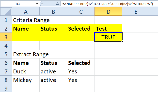
– data capture-data view.JPG: this shows a portion of the sheet where I’m capturing the results of Test 1. The formula to capture the data uses info about what sheet and column to get the data from; that way I can use the same formula for all the types of grades (tests, quizzes, etc)
– data capture-formula view.JPG: this shows the formulas involved in the above. See the formulas in C16:C17 (“approach 1”) vs those in C18:C20 (“approach 2”)

Basically “approach 1” uses the ADDRESS BIF to put together the input for the INDIRECT BIF; “approach 2” puts together the input by concatenating the pieces needed by the INDIRECT BIF. Both use the MATCH BIF to find the proper row in the “tests & grades” sheet for the student named in Col B; both also use a +15 since student names start in row 16 of the “tests & grades” sheet, whereas MATCH is returning a relative number within the range $A$16:$A$47 where student names are located. Once the correct row for “student1” etc is found, the column where his/her test1 grade is used to find the grade.

In this way, the same formula can be used for all students and for all types of assignments to populate the spreadsheet that Canvas exports and re-imports. I don’t have to enter individual grades back into Canvas, since my gradebook already has the data; I can just copy/paste the grades from the sheet shown in the captures into Canvas’s spreadsheet and then re-import to Canvas.
Any ideas on how to improve the formula? Any thoughts on which of the existing formulas/approaches is better? In terms of “better,” issues of extensibility come into play and affect of the formula on size of the file (probably not a big deal); I’m not too concerned about execution time since grades, once assigned, are not likely to change.

One thought that I had is to treat the various sheets like “tests & grades” as a giant lookup table, use that to find the proper row for the student and tell VLOOKUP to return the value from the appropriate column.

And if you want to know why I don’t just input my grades directly into Canvas, that’s for a different time (and not on this Lounge).

TIA.

Fred

Reply | Quote

Replies

Happy New Year to you.

You did not say which Excel your running so I hope its 10 or above.

After looking at the problem my recommendation is to abandon all the complex formulas. Instead use the power of advance filter to find and retrieve the information. To do this you will need to do the following

1. Create a range name for the grades worksheet large enough to include both current and future expansions
2. Create the Criteria for the data you want
3. Create the Exact Column names for the desired output
4. When running the Advance Filter make sure to select “Copy to another location.
5. Run the Filter and the results will be at the Copy Location Selected

Attached is an example, to run the advance filter. Make sure to type the range name “Groups” then check the box to copy to another location then run. Results will be there. Change the Criteria name to “Test 2” and run advance filter and see the new results

I think this may be better since everything is being run by “Criteria” that is part of excel which you can quickly change. Far more flexible.

Lastly, as long as the criteria is correct the results are values rather than complex formulas. This should keep the file from getting too large and allow for quick access to any data in the grades database.

Hope this helps.

TomD

Reply | Quote

Tom – forgot to mention in my previous post: I’m running Excel 2003 (Version 11). Is version 10 the first version with Advanced Filtering?

Reply | Quote

Hi Tom,

Thanks for the suggestion. We just got back from a few weeks of vacation and have been slowly catching up with all that happened while we were gone.

One of the problems I’ve always had with Advanced Filter is that it’s not dynamic when using the copy to another location. I think in this case, that may not matter.

I ran a brief experiment and I can see that this could work. One question on the criteria:
– what I would prefer for some of the sheets needing filtering is a criteria that says to select those rows where a certain column contains something OTHER THAN the phrases “too early” and “withdrew” (w/o the quotes). I tried setting this up as “too early” in one column and “withdrew” in an adjacent column with the same heading. Didn’t work. So I resorted to having 6 rows for what the column could be and that worked fine.

Any suggestions to how to set up what I do want?

But for other sheets where those phrases don’t appear, I would have to resort to creating a new column with data from another sheet that provides the filtering criteria.

And it certainly does look like the size of my spreadsheet has grown quite large. I’d almost be willing to be that the Advanced Filtering would reduce the size of the file.

Thanks.

Fred

Reply | Quote

Fred,

See if this meets your needs?

Sample DB:
43448-FredDb

Criteria & Extract Ranges:
43451-FredResults

Now take note of the CRITERIA field that is NOT part of the database! Yeah, I was taught you couldn’t do this but not so.

So in this made up field name you can put any valid Excel formula that will evaluate to True/False.
In constructing this formula refer to cells in your FIRST DATA ROW!

Thus in this example we use [noparse]=AND(UPPER(B2)”TOO EARLY”,UPPER(B2)”WITHDREW”)[/noparse]

And viola! you only get the ones you want. BTW: Tested on 2010 & 2003.

Test File: 43450-Advanced-Advanced-Filter

HTH :cheers:

May the Forces of good computing be with you!

RG

PowerShell & VBA Rule!
Computer Specs

Reply | Quote

Hi RG,

I think what you did would work. For some reason, I also had it working with my current layout when I tried Tom’s suggestion; the layout included some blank columns and some duplicate column names. Now I can’t get it to work – I get the infamous “The extract range has a missing or illegal field name.” I can’t quite figure it out but not sure it’s worth trying.

I was taught like you – everything on one sheet. I think as long as the Criteria and Extract Ranges are on the same sheet, it doesn’t matter what sheet they are on relative to the DB.

Fred

Reply | Quote

Fred,

I find if you use Named Ranges for Database, Criteria, and Extract it doesn’t much matter. If you check the sample you’ll see I used those names. The other thing I ALWAYS do is to use References for the column names in the Criteria and Extract ranges pointing back to the Database headers. That way you don’t have to worry about spelling mistakes which cause the “The extract range has a missing or illegal field name.” messages.

HTH :cheers:

May the Forces of good computing be with you!

RG

PowerShell & VBA Rule!
Computer Specs

Reply | Quote

Thanks RG.

I tend to copy/paste the column headings from the DB to the Criteria Range. I either do that or use references for the Extract Range.

I think my problem was the blank and duplicate column headings I had within my DB.

I don’t quite recall how I got it to work the first time. When I did it this last time, I used my tests sheet – where I do have blank cols and duplicate col headings. I thought I used my tests sheet before also but it could have been my quizzes sheet where there are neither blanks nor duplicates (I really don’t think so but…).

Anyway, I decided on kind of a compromise approach for now kind of inspired by the Advanced Filter approach.

My grades are stored on different sheets: one for tests, one for quizzes, one for projects, etc. So, using Advanced Filter would necessitate having a “setup” on each sheet – at least from what I can see. Each sheet has a different number of possible grades: quizzes have a max of 10, projects have 4, and tests have 3 or 4 depending on the class.

I originally took a brute force approach based on what I posted on Jan 1 and the formulas there. Every quiz (up to 10 even if I only gave 8 quizzes in the semester), every project, every test, etc. were present on the sheet (the one that I’d use to copy/paste to the Canvas spreadsheet) but only for ACTIVE students. This even though I would probably only be pasting one or two assignments (one quiz and maybe a project) after a given class. The file size, with formulas like I showed in post #1, grew to 1.2MB with no student data in it.

One of the reasons for the extra formulas was that I wanted all data for a given assignment in one contiguous set of rows ONLY for ACTIVE students. When I paste to the Canvas spreadsheet, it only has rows for ACTIVE students. Even if a student withdraws, I keep them in my gradebook where they were. So the quizzes and tests sheets have rows alphabetically for all students regardless of whether they’ve withdrawn or not. If I pasted my original data to the Canvas spreadsheet, I’d paste, say, 3 consecutive rows for 3 ACTIVE students, then skip the next 2 rows in my spreadsheet, copy another 2 rows for the next 2 ACTIVE students, etc (or just paste everything and then start moving grades up for only the ACTIVE students).

What I decided to do is just have 1 column for grades on the new sheet (call it the “Canvas Interface” sheet) rather than just 1 column for each possible grade. This is next to a column of names, which only has ACTIVE students. By way of a drop-down box and a small lookup table, I can say what kind of assignment (quizzes, tests, etc) I want and the number of the assignment (so Test 1 or Quiz 3). Using this info, I can fetch the grades for just the ACTIVE students for just that assignment. I can then paste these into the Canvas spreadsheet at one time. If I have a second assignment that was done that day, I just change the assignment type and number info and I’m ready to paste again. Then I import the Canvas spreadsheet into Canvas and I’m done – students can see their grades. My spreadsheet is now just 980KB.

Thanks for all the help.

Fred

Reply | Quote

Fred,

Glad you got it sorted to your liking and glad to be of assistance. :cheers:

May the Forces of good computing be with you!

RG

PowerShell & VBA Rule!
Computer Specs

Reply | Quote